SOLIDWORKS Simulation vs Abaqus: When Should You Upgrade?

The engineering design process can take a wide range of paths when creating a new product. During the initial conceptual stage, designers and engineers generally start with a set of initial calculations using “back of the envelope” methods to determine if a design is feasible. These calculations are based on industry standards, typical assumptions, and idealizations which make them quick and simple to perform. 

As a design progresses, engineers move on to more detailed analyses to validate the design. This is where SOLIDWORKS Simulation can be leveraged to quickly analyze individual components and multi-part assemblies in a range of loading conditions. 

Because of the user-friendly interface and tight integration with SOLIDWORKS CAD, engineers can quickly iterate through multiple configurations or potential solutions before pushing their changes to production. In general, SOLIDWORKS Simulation is ideal for the conceptual design stage and can handle analyses including linear static, nonlinear static, and specific dynamic simulations. Beyond that, with SOLIDWORKS Simulation, one can perform topology, fatigue, and thermal analyses, thus allowing them to answer a wide range of design questions with a single tool. 

However, as designs become more complex, the limitations of SOLIDWORKS Simulation become apparent, and more powerful tools like Abaqus are required. In this article, we'll compare SOLIDWORKS Simulation and Abaqus and discuss the following topics: 

Table of Contents

• SOLIDWORKS Simulation vs. Abaqus Comparison
• Control in Mesh Generation
• Customization of Material Models
• Loading Approach
• Explicit Dynamic Simulations
• Contact Modeling
• Parallel & Cloud Computing
• License Approach
• Test Problem Comparison
• Results Comparison
• Mesh Convergence Study
• Conclusion

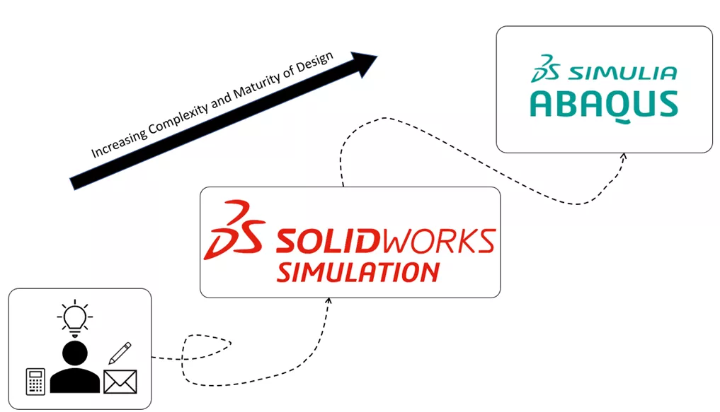
Figure 1: Idealization of the Maturation of an Engineering Design

In general, Abaqus allows for a higher level of fidelity and accuracy in simulations due to the ability to fine-tune mesh controls, a diverse selection of specialized element formulations, and numerous complex material models. Beyond that, the ability to represent multiphysics scenarios can allow engineers to capture interdependent phenomena seamlessly. 

In short, the engineering design process typically moves from the back of the envelope calculations to conceptual design and simulation with SOLIDWORKS Simulation. From there, the design can transition to Abaqus when it becomes sufficiently mature and complex. Both tools come with a large community of users that can offer varying approaches and insights to a problem via online videos, blogs, forums, and training courses. Each comes with its strengths and weaknesses, and the choice of tool will depend on an engineer’s individual project needs and the stage of the design cycle they are currently in. 

SOLIDWORKS Simulation vs Abaqus Comparison

To compare SOLIDWORKS Simulation and Abaqus, we’ve created a matrix that highlights their strengths and weaknesses: 

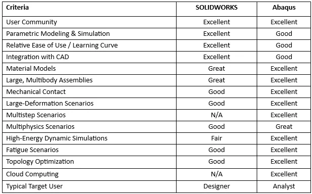
SOLIDWORKS Simulation & Abaqus Main Differentiators 

Control in Mesh Generation 

Figure 2: Representation of 1 ^st order tetrahedral (left) and 2 ^nd order tetrahedral (right). These are the style SOLIDWORKS Simulation uses for 3D solids

When generating a mesh during the pre-processing stage, SOLIDWORKS Simulation is capable of creating 1D beam elements, 2D triangular surface elements, and 3D tetrahedral solid elements. From there, elements within SOLIDWORKS Simulation can be subdivided into either draft-quality linear elements or high-quality quadratic elements (also called 1st order and 2nd order, respectively). The main trade-off between the two is accuracy and computational efficiency.

SOLIDWORKS Simulation offers automatic mesh generation, which can be useful for quickly generating a mesh for simple geometries. However, for more complex geometries, users may need to spend more time manually creating and refining local distributions of the mesh to obtain accurate results. 

Figure 3: Representations of 1st order (left) and 2nd order (right) hexahedral elements. Abaqus is capable of using hexahedral and tetrahedral elements to represent 3D geometry

Conversely, Abaqus offers a wider range of options and controls for users to create high-quality meshes that can accurately capture the behavior of complex geometries and loading conditions. With the pre-processing tool  Abaqus/CAE, engineers have access to a variety of meshing schema, which generally falls into categories of structured, unstructured, and hybrid. 

Similar to SOLIDWORKS Simulation, users can create 1D beams, 2D surface elements, and 3D volumetric elements within Abaqus/CAE. However, a key difference is the support for 2D quadrilateral surface elements and 3D hexahedral elements within Abaqus. In general, hexahedral elements tend to be more computationally efficient and require fewer elements to accurately capture similar loading responses when compared with tetrahedral elements. However, the performance of each element type is largely driven by the scenario in which they are being applied.  

Figure 4 : Comparison of Tetrahedral and Hexahedral meshes during a drop test scenario

Above is a comparison showing the performance of linear tetrahedral and hexahedral elements subjected to a drop test within Abaqus/Explicit. 

In this comparison, the impact of the drop creates a planar compressive wave that propagates upwards through the solid. Once the planar wave reaches the top boundary of the solid, the reflecting wave decomposes into a mixture of constructive and destructive interference patterns as reflections off the sides of the solid begin to interact. 

This interference pattern is more recognizable in the hexahedral mesh as the results maintain a degree of symmetry throughout the scenario that is not held by the tetrahedral mesh. When viewed side-by-side, the tetrahedral mesh shows a greater amount of numerical noise in the results. 

Customization of Material Models 

For users looking to answer more fundamental questions of their design, like, “Will my component yield under this tensile load?” SOLIDWORKS Simulation has a fantastic Material Library to quickly pull material properties for use in simulation. Additionally, users can create custom materials with models ranging from simple linear elastic isotropic metals to nonlinear hyper-elastic rubbers. This covers a large portion of the needs for analysts; however, limitations tend to arise in the material model capabilities when material nonlinearities need to be accounted for. 

Abaqus takes a different approach than SOLIDWORKS when it comes to material modeling. Rather than offering a database of pre-defined materials for users to pick and choose from, Abaqus offers numerous material models that can be fine-tuned to a user’s needs based on the material properties they choose to assign. For simple linear elastic isotropic metals, this is functionally the same as SOLIDWORKS, provided the Young’s modulus and Poisson’s ratio are equivalent between the two programs. 

Abaqus exceeds SOLIDWORKS in its capabilities to accurately represent material nonlinearities such as damage accumulation, fracture mechanics, element deletion, and even discrete element methods for highly nonlinear applications. This is useful for analysts looking to tune material models to specific material data collected from physical testing for use in simulation.

Figure 5: Charpy impact test using an element deletion material model. Watch elements disappear as stress increases!

While both Abaqus and SOLIDWORKS Simulation offer a range of material models, Abaqus provides more advanced features for the customization and modeling of nonlinear material behavior. In short, if a user is simply looking to answer the question of “Will my steel truss yield under these static loading conditions?”, SOLIDWORKS is more than capable of producing answers in an efficient manner. When complexity arises, such as the simulation of an impact analysis of that steel truss, users may need to look towards a more powerful tool such as the  Abaqus/Explicit solver. 

Loading Approach 

Within  Abaqus, a core feature to the setup of an analysis is the concept of a step. Within a given simulation, users can sequentially link multiple analysis steps of varying types together. A common example: 

• Step 1: Extraction of Natural Frequencies for a structure in a base state. 
• Step 2: General static step including nonlinear geometric considerations, where stress develops. 
• Step 3: Extraction of natural frequencies to display the effects of the stress state. 

This stepwise loading approach is integral to the analysis setup and allows users to chain together numerous combinations of analyses to answer niche questions for a particular design.  

Additionally, users can utilize this stepwise loading approach to accelerate particular scenarios if they leverage restart analysis capabilities within Abaqus. Imagine if a user had a coordinated and extensive pre-stressing routine as loads are sequentially applied, followed by the investigation of multiple load cases where a load varies in amplitude, direction, and point of application.

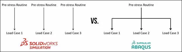
The first stage of the analysis could be performed once with restart information requested. Following that, every branch of the possible amplitudes, directions, and points of application could be run using the first restart analysis as a seed for the follow-on simulation. Thus, the user could skip running the pre-stress routine every time, resulting in a much faster runtime in the coverage of all possible load cases. 

There are some limitations on what analyses can be linked together. For example, there's a short additional process in order to follow up an Abaqus/Standard static general step with an Abaqus/Explicit dynamic step, as the two utilize two different solving utilities. In order to do this, the user must perform an Import analysis to translate the current stress state and geometric information from one solver to another. Swapping between the Explicit and Standard solver within Abaqus can be very powerful for certain analysis applications such as a metal-forming and spring-back investigation.  

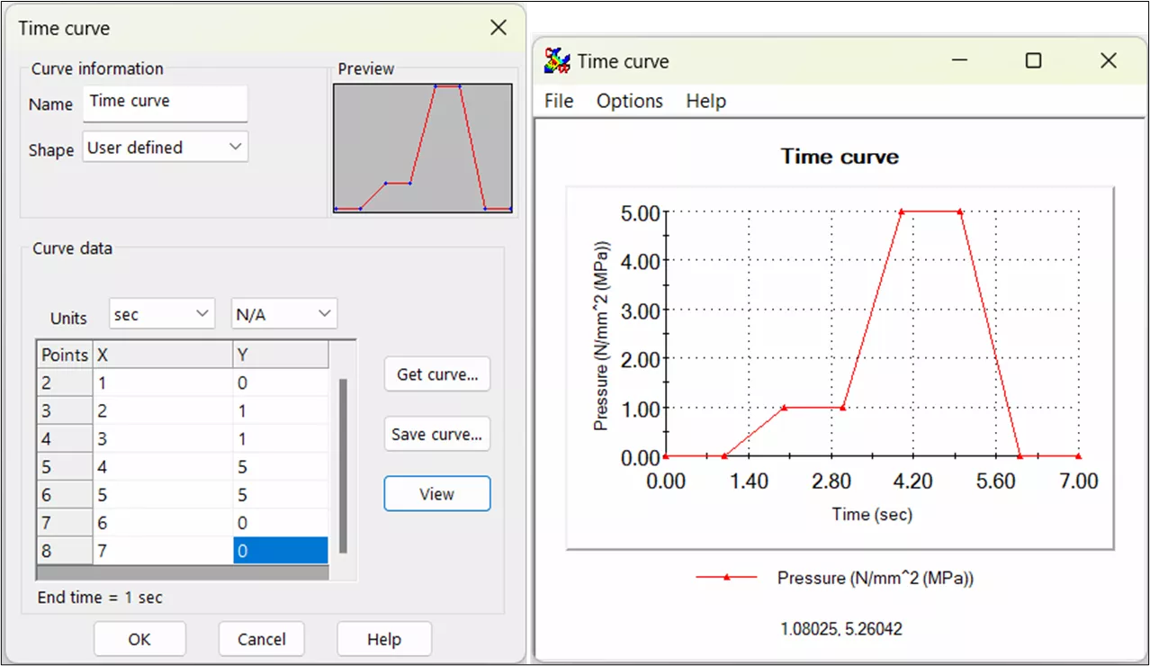
Figure 6: A time-curve for a pressure load built in SOLIDWORKS. Transition between datapoints is always linear. There is no way to continue a partially completed calculation

SOLIDWORKS Simulation, on the other hand, does not take a stepwise loading approach. Rather, in order to coordinate multiple loading conditions to be applied sequentially, the user must declare several time curves. These time curves allow the user to control when loads are applied to the structure but do not give the user as much control as the stepwise loading schema does within Abaqus. Additionally, restart analyses are not available within SOLIDWORKS Simulation. 

Explicit Dynamic Simulations  

Figure 7: Example of an explicit dynamic simulation using the Abaqus solver

Explicit dynamic simulations are typically used to represent the response of a structure to a high-strain rate and high energy density loading condition. Loads in these scenarios can be applied at a rate comparable to the first natural frequency of the structure. In contrast to static simulations, values for velocity and acceleration do not have to equal zero over the course of the simulation and thus considerations for inertial and damping forces tend to arise. Common simulation routines include virtual drop tests, blast wave analyses, and impact analyses.  

Within SOLIDWORKS Simulation, one can create explicit dynamic simulations, but only in a narrowly defined sense. Drop test studies use an explicit solver, but are limited to rigid materials, no virtual connectors, and solve time considerations. An implicit dynamic solver is available in Nonlinear studies. Limitations arise in SOLIDWORKS Simulation due to shortcomings of high strain-rate behavior in material models as well as inadequacies in mechanical contact which can lead to nonphysical results.

In contrast, Abaqus offers a highly advanced and efficient explicit dynamics solver. Simulations that recreate complex contact interactions, extreme deformation, and large-scale material failure are well suited for the Abaqus/Explicit solver. Within this tool, a myriad of utilities are available to represent a number of complicated situations. If a user expects incredibly high deformation of their mesh during a press-forming simulation, they can leverage the Coupled Eulerian Lagrangian (CEL) mesh technique to introduce stability in the forming process. Element deletion exists as a way for users to remove material from a simulation, potentially as a way to represent spalling and material ejection during an impact analysis. General contact can be used to represent the interactions of multiple bodies quickly and easily within a domain without specifying all possible contact pairs manually.  

These examples merely scrape the surface of techniques available to a user with the Abaqus/Explicit solver. Because of its stability and accuracy, the Abaqus/Explicit solver is a tool that is widely implemented in projects within the aerospace, automotive, and defense industries where considerations for dynamic events can shape the nature of a product. Overall, Abaqus/Explicit is a more comprehensive and sophisticated solver compared to the routines available within SOLIDWORKS Simulation. 

Contact Modeling  

Figure 8: Example of general contact within Abaqus/Explicit study. Almost a strike!

Contact modeling is a means of representing the interaction of separate bodies as they pass forces and pressures between one another. Simple contact interactions typically involve a certain amount of normal force being passed from one body to another in order to prevent mesh penetration, as well as the development of friction forces to resist unconstrained sliding of one mesh on another. 

Both SOLIDWORKS Simulation and Abaqus include contact modeling algorithms to represent this phenomenon of structural mechanics. 

SOLIDWORKS Simulation offers a penalty-based contact method that introduces stiffness and a restoring force between surfaces whenever penetration is detected during the solve. This method is a simplified approach to contact modeling and can give realistic results, provided a proper penalty stiffness is chosen. 

If stiffness is too low, bodies can penetrate one another leading to non-physical simulations. On the contrary, if stiffness is too large, artificially high stresses can be reported. A limitation of SOLIDWORKS is the sole reliance on the linear penalty method as an enforcement mechanism. 

This is contrasted with Abaqus and its ability to use additional enforcement mechanisms such as a tabular overclosure-pressure relationship, a non-linear penalty method, or the Lagrange multiplier method. Abaqus provides more flexibility in the number of approaches available if non-physical results show up in a contact simulation. 

Another key advantage for Abaqus is the previously mentioned general contact algorithm. With this tool, users can define all bodies to be included in the contact domain, prescribe a set of contact enforcement properties, and run the simulation. 

In the below animation, the general contact domain is specified with two features added to the simulation, rather than needing to specify the potential for interaction of each pin with each other.  

Figure 9: (Top-view) Example of general contact within Abaqus/Explicit study. Almost a strike!

Where SOLIDWORKS Simulation users would otherwise need to specify every potential contact pair manually and troubleshoot mesh penetration, general contact and Abaqus’ enforcement properties are major time-savers in situations where multiple bodies or internal faces collide. 

Parallel & Cloud Computing 

As a finite element model becomes larger and includes vast quantities of nodes and elements, parallel computing becomes a powerful strategy to manage the long solve times. 

Within SOLIDWORKS Simulation, users can run multicore solves; however, a key limitation is that SOLIDWORKS Simulation’s parallelization plateaus at a relatively low number of cores compared to the core counts available on the CPU market. Additionally, multi-socket and distributed computing methods are unsupported.  

Abaqus, on the other hand, has a robust parallel solver that can effectively leverage high-core-count CPUs, multi-CPU workstations, local HPC clusters, and cloud compute environments. This allows users to run much larger and more complex simulations while significantly reducing the solve time. In order to solve with multiple cores users will need to have a pool of tokens sufficient to support the license requirement, where large parallel simulations require more tokens to run than simple single-core simulations. You can read more about this in the licensing section of our Abaqus Buying Guide. 

License Approach  

SOLIDWORKS Simulation offers three levels of licensing, including Simulation Standard, Simulation Professional, and Simulation Premium. Each license offers different capabilities and solvers. 

The entry point Simulation Standard license offers static analysis for linear-elastic materials. This license creates an attractive entry point for users looking to incorporate basic FEA into their design process, answering design questions like, “If I add a new stiffener to this design, how much does it limit elastic deformation?”. 

On the other side of the licensing hierarchy, Simulation Premium gives access to linear dynamic, nonlinear, thermal analyses, and more. As the user requires more advanced simulations, they’re able to upgrade to the next level of solvers within SOLIDWORKS Simulation. 

In contrast, Abaqus takes a Unified FEA approach where if a user purchases a license, they are able to run any and all analyses supported within their particular version. Abaqus licenses are also network-based, so the preprocessor and solver are not tied to any physical machine. An Abaqus purchase also includes access to fe-safe and Tosca Optimization Suite for fatigue and topology optimization, respectively. While they are their own separate programs, they run off of Abaqus analyses and use the very same licenses. During the purchasing process, users will discuss their current and future simulation needs with GoEngineer, and GoEngineer will put together the most effective and affordable licensing options for the user to choose from. 

Test Problem Comparison 

To highlight the similarities and differences between Abaqus and SOLIDWORKS Simulation, we’ve prepared a simple test model to be simulated in both programs. 

In this model, we have two metallic plates with dissimilar coefficients of thermal expansion that are held together by four stainless steel bolts. The loading scenario considered involves a 500 Newton preload applied to each of the bolts, followed by an adiabatic change of model temperature to capture stresses induced by thermal expansion. The temperatures considered for the thermal expansion analysis include a high-temperature condition (+200 C) and a low-temperature condition (-100 C). Due to a difference in thermal expansion coefficient for the two plates, the change in temperature will drive a misalignment of the bolt holes and create a rise in stress for the two parts. General or global contact will be used in both simulation software creating non-penetration conditions. No friction has been modeled between the plates. 

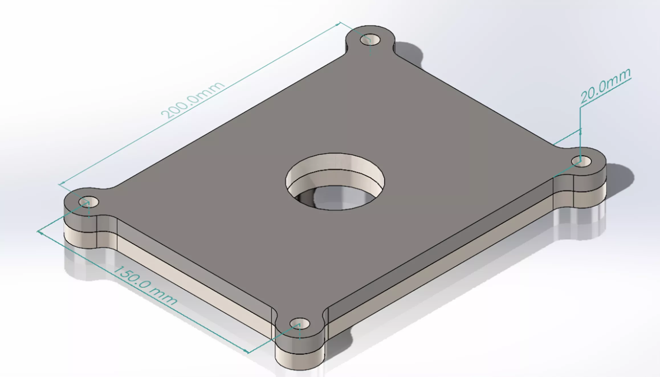
Figure 10: Overview of geometry to be utilized in test problem

In this case, a doubly symmetric model can be created which allows us to simulate only a quarter of the total model. This provides both the benefit of computational efficiency as well as the recovery of symmetric results about the two primary planes of symmetry. 

Boundary Conditions  

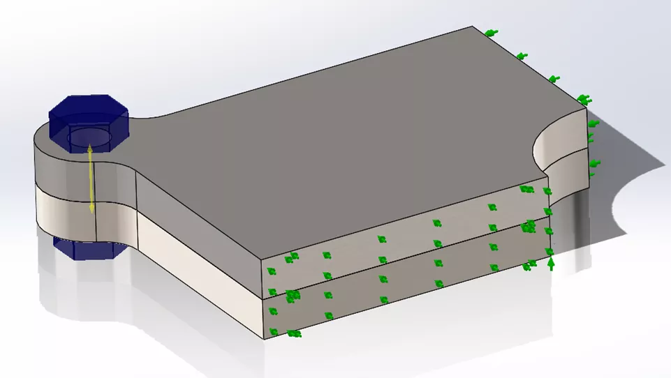
Figure 11: Depiction of quarter-model within SOLIDWORKS Simulation

In order to properly constrain this model for a general static analysis, one must provide adequate boundary conditions throughout the model to prevent unconstrained rigid body motion. However, if one over-constrains the model, unrealistic distributions of stress can arise. For a thermal expansion analysis, the use of the 3-2-1 rule of fixturing is helpful in developing a set of minimally restrictive constraints. This allows the body to deform more freely about a single reference point. Identical boundary conditions are provided for the SOLIDWORKS Simulation and Abaqus models to create a fair comparison. 

In this case, we’ve utilized two planes of symmetry that each remove one normal translational degree of freedom and two rotational degrees of freedom about the normal direction of each symmetry plane. Thus, the only remaining primary direction to be constrained is parallel to the bolt-axis. This final constraint is created by applying a zero-displacement condition for a vertex of the center hole in the bottom stainless steel plate. 

Material  Properties  

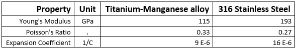
For this simulation, two materials have been pulled from the SOLIDWORKS material library. For this simple scenario, only three properties are required to fully characterize the response. Because the scenario is adiabatic and temperature is linearly ramped in a global sense, considerations for specific heat, thermal conductivity, and mass density are not required. Thus, all the solver needs in either software is a quantity for thermal expansion coefficient in order to determine nodal displacements.  

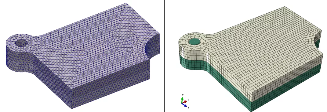
Figure 12: Side-by-Side comparison of SOLIDWORKS tet-mesh (left) and Abaqus hex-mesh (right)

Shown on the right, is the first-order, linear hex-dominant mesh generated for the Abaqus simulation with a target element size of 2.5 millimeters. Given the rectangular shape of the overall geometry, a hex-dominant mesh fits well. A local mesh refinement about the bolt hole has been specified to emphasize the curvature of the opening. Because of this, some wedge elements have been generated to limit any skewed elements that might otherwise have been generated in a hex-only mesh. With this target element size, the node count reaches approximately 12,500. 

Shown on the  left , is a first-order, linear tetrahedral mesh generated by SOLIDWORKS, also with a maximum element size of 2.5 millimeters. The elements follow the curvature of the holes using the “blended” automatic mesher, but sacrifice the symmetry capable of the hex elements. There is also a slight sacrifice in solve time, as the node count is over 15,000.  

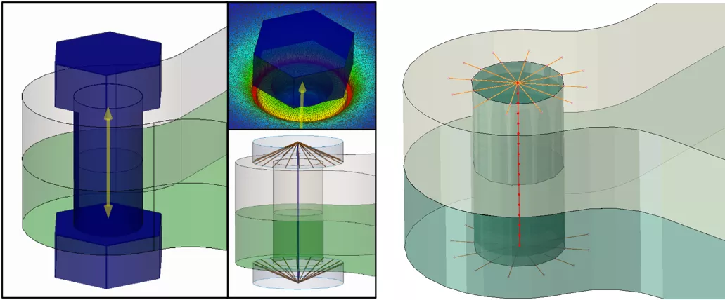
Figure 13: SOLIDWORKS bolt connector, exaggerated deflection due to pre-load, and imagery describing the bolt connector formulation (left). Additionally displayed is a virtual bolt created using a combination of distributed couplings and beam elements in Abaqus (right)

Within Abaqus, several approaches exist for the creation of a virtual bolt which, broadly speaking, fall into two categories of representing the shank of the bolt. Either one can use a singular connector element to prescribe the relation between two reference points of couplings, or one can create a line and discretize using 1D beam elements. In this case, the bolt is represented via a combination of 1D beam elements and distributed couplings. 

To represent both the bolt-head and end-nut, a distributed coupling was implemented to constrain the degrees of freedom down to a central reference point. From there, a 1D beam mesh was generated with a circular profile to represent the shank of the bolt. This methodology was chosen so that a 316 stainless steel material section could be applied to the bolt shank. This allows us to consider the influence of temperature on the expansion or contraction of the bolt itself with respect to the temperature change.  

The virtual bolt connector in SOLIDWORKS allows us to apply a preload to a virtual connector, compressing the plates together. SOLIDWORKS represents this bolt as a singular connector element through the shank, and in this case, uses rigid connectors to connect the connector element to a circle representing the bolt head and nut. 

The SOLIDWORKS virtual bolt also uses 316 stainless steel and maps over the temperature distribution of the surrounding plates, but is only able to expand axially, not radially. Finally, SOLIDWORKS either has the choice to assume the bolt shank is fit tightly within the holes, or as in this case, is a loose fit. In the case of a loose-fit bolt shank, the internal vertical face of the bolt hole is unconstrained with respect to the shank and can deform independently from the shank. 

Results Comparison 

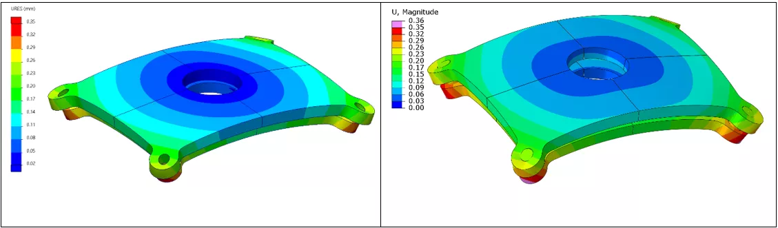
Figure 14: Low-Temperature Displacement results for SOLIDWORKS (left) and Abaqus (right)

Shown above are the results of the thermal expansion simulation in the low temperature (-100 C) scenario. Displacements have been scaled by a factor of 100 to visualize the manner of deformation between the two plates. In the low-temperature scenario, the stainless steel plate on the bottom of the stack contracts at a faster rate than the titanium alloy on top. This results in the convex shape as displayed and a maximum displacement of around 0.35 millimeters. 

In a broad review of the results, the two distributions of displacement are comparable and on the same order of magnitude. Both solvers agree that the level of maximum global displacement is around 0.35 millimeters. If one looks at this metric alone, the over-arching takeaway would be similar; however, upon closer examination, the results generated from the Abaqus simulation appear more realistic, particularly as it relates to the interaction around the bolt hole. 

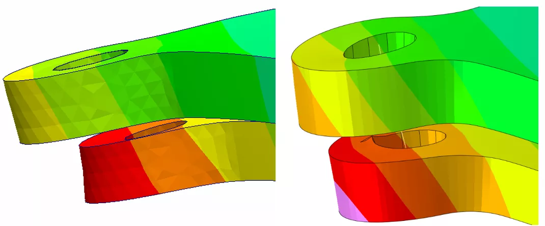
Figure 15: Low-Temperature Displacement results at 100x scale for SOLIDWORKS (left) and Abaqus (right)

When scaled by a factor of 100, some level of misalignment is expected due to the elastic deformation of the bolt shank; however, the results gathered from SOLIDWORKS Simulation indicate a much higher level of misalignment than the Abaqus simulation. This is likely due to the inclusion of the beam elements in the general contact domain within Abaqus. This interaction of the shank with the bolt hole restricts the misalignment. SOLIDWORKS Simulation does not consider connector-to-surface contact which leads to a higher degree of misalignment. Additionally, because a loose fit was chosen for the SOLIDWORKS virtual connector, the bolt holes are allowed to expand more freely relative to one another compared to the implementation in Abaqus. 

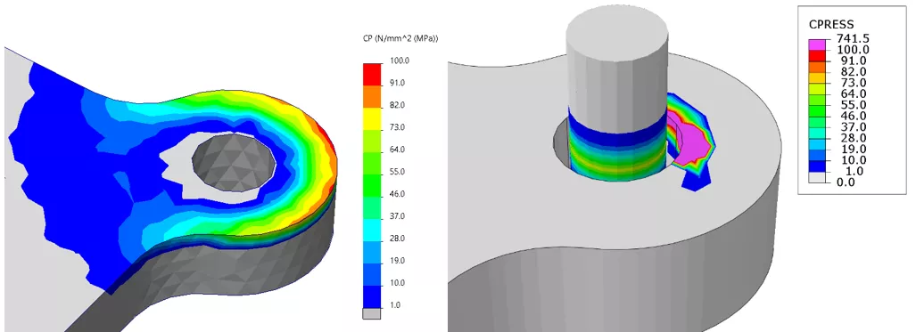
Figure 16: Low-Temperature Contact Pressure results on the lower plate for SOLIDWORKS left) and Abaqus (right). The beam profile in the Abaqus results has been scaled by 0.75x for post-processing visualization

When comparing contact pressure, the results differ substantially due to the inclusion of the beam elements in the Abaqus general contact domain. When the beam profile is scaled by a factor of 0.75, one can see the development of contact pressure about the center of the shank where it presses into the top edge of the stainless steel plate. Without this restricting contact interaction, SOLIDWORKS indicates that the surface-to-surface contact is the limiting factor for the deformation of the plates. In this scenario, the approach taken in the Abaqus simulation is more realistic as the shank occupies physical space and will create mechanical interference upon deflection. 

Mesh Convergence Study 

A common practice within Finite Element Analysis is the performance of a mesh convergence study (also referred to as a mesh refinement study), where the user continuously refines the mesh and tracks the output variable of interest. Barring any modeling errors, as refinement increases, the solution to an FEA simulation should converge closer to a consistent, mesh-independent value. This increase in accuracy comes with a sacrifice of computational efficiency, where every additional refinement vastly increases the solve-time while only marginally changing the output value of interest.  

In this scenario’s case, a mesh convergence study was performed varying the target element size from 10 millimeters at the largest down to 1.25 millimeters at the smallest. The solvers were tested using both linear (1st order) and quadratic (2nd order) elements. The output variable of interest tracked was the global maximum displacement for the assembly at both the high-temperature condition (+ 200 C) and the low-temperature condition (-100 C). 

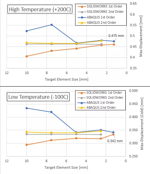
In this analysis, both solvers converge to approximately the same value of 0.475 millimeters for the high-temperature condition (+200 C) and 0.342 millimeters for the low-temperature condition (-100 C). As expected, the 2nd order elements for both solvers reached the converged value sooner than the 1st order elements. Due to the higher solve-time of the 2nd order elements and sufficient justification for mesh-independence, the 2nd order mesh convergence study was run only to 2.5 millimeters for both solvers. 

Abaqus' first-order hex elements began to match second-order hex elements at 5mm. Using 4-cores for computing, the results took 37 seconds to calculate. SOLIDWORKS Simulations' 1st order tetrahedral elements began to match 2nd order tetrahedral elements at 1.25mm. Using a 6-core machine for computing, the results took 191 seconds to solve. 2nd order elements for both solvers produced reasonably precise displacement results at 10 millimeters, both taking approximately 20 seconds to solve.  

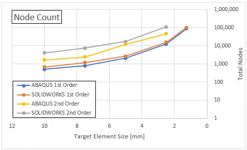
Shown above is a depiction of the number of nodes generated in the assembly as a function of the requested target element size. As the requested target element size becomes increasingly small, the number of nodes skyrockets, as depicted by the non-linear growth on a logarithmic Y-axis. Additionally, it can be seen that 2nd order elements generate approximately a 5-fold increase in the number of nodes. This directly contributes to the higher solve times required for 2nd order elements as the number of degrees of freedom in the model directly correlates with the number of nodes.  

The other key piece of information is the lower node count for hex-elements (Abaqus) in both the 1st order and 2nd order elements. Without digging too far into the details of solver differences or the considerations of optimized parallel computing environments, what can be seen here is that a lower node count from the hex-dominant mesh can lead to faster solve times while delivering accurate results. 

Conclusion

FEA Tools Make Approximations – Take Care to Understand their Effects

For every job, there is a proper tool. Through this test case, we’ve shown that SOLIDWORKS Simulation makes for an adequate high-level simulation software capable of providing accurate answers to over-arching questions at this subassembly scale. This can be seen by the validation that is achieved in the global displacement metric between the two solvers as they converge to a similar solution. If this is the sole metric that judges the efficacy of a component or design, then SOLIDWORKS Simulation can provide the answer to that narrowly defined question. However, the results taken away from any FEA software need to be viewed in light of the approximations made during the solve. With SOLIDWORKS, particularly as it relates to contact problems, one must be aware of the limitations and assumptions that influence how their results can be interpreted. 

More Complexity Will Require Abaqus

Additionally, this test problem exists at the crossroads of complexity for the two solvers and was designed to be doable in both. However, if this problem’s definition were to be expanded to include a soft rubber gasket between the two plates, a much higher preload in the bolts, and/or an internal fluid cavity pressure applied to the center hole, SOLIDWORKS Simulation may struggle to produce accurate results. Furthermore, if this two-plate component was one subassembly on a much larger assembly, a high-core-count or GPU-accelerated workstation or cloud compute would be necessary to provide results in a timely manner. Because of its nature as a highly-scalable finite element solver, Abaqus picks up and becomes a much more effective solution where SOLIDWORKS begins to run into its limitations.

Abaqus Can Push Your Products – and Your Innovative Leaps – to their Limits 

Abaqus is the next step in the engineering design process after SOLIDWORKS Simulation. When looking to evaluate and diagnose failure points within a multibody design subjected to a wide variety of loading conditions, Abaqus provides a much more powerful suite of tools for the user. When properly implemented, Abaqus can make for a holistic approach to a simulation-driven modeling environment.

How to Get Started with abaqus

Our product pages for traditional Abaqus and 3DEXPERIENCE STRUCTURAL (which is essentially Abaqus on the 3DEXPERIENCE Platform) are a great place to start learning more about Abaqus. Our Abaqus buying guide also answers many frequently asked questions about the software, buying process, packaging, licensing, cloud capabilities, and more.

You can also simply contact us for a personalized, guided introduction to Abaqus as it relates to your business, informed by our many years of experience as a simulation consultancy.

Lastly, even if you're not ready to own Abaqus, you can still take advantage of many of the benefits discussed here on a per-project basis by leveraging our advanced FEA services, for which we primarily use Abaqus.

Related Articles

The Ultimate Guide to Abaqus Computing

Computational Fluid Dynamics (CFD): Applications & Solutions

Abaqus and CATIA Now Available from GoEngineer: NOT Just for Enterprise!

Thermal Analysis Using SOLIDWORKS: FEA vs CFD

VIEW ALL ARTICLES