FEA Materials Are Make-or-Break: Introducing the 3DEXPERIENCE Material Calibration App

Finite Element Analysis (FEA) tools like Abaqus/Explicit or the 3DEXPERIENCE Platform provide a fantastic solution if you’re looking to investigate your product’s performance in simulation before spending the resources to develop a physical prototype. But for those that adopt these tools, there can sometimes be the hurdle of material modeling and its influence on your simulation’s ability to predict reality. Using improper material properties can lead to drastically different conclusions in your FEA simulations if you’re not careful. Throughout this blog, we’ll demonstrate what might happen to you and your product should you skip over the time and effort required to develop a proper material model for your scenario.

Running material tests on your product will always be a recommended course of action if you are seeking fully validated results. These tests provide the best insight into the stiffness, strength, and other characteristics that may be influenced by manufacturing processes, supplier differences, and environmental factors.

Suppose you run your material tests and have successfully collected a pool of stress-strain curves that cover the anticipated loading conditions your product may be exposed to. The issue now stands at how best to leverage that data and how to formulate it in a way that your simulation can accept it.

For years, the solution to this in many companies was to develop a set of complicated Excel workbooks that would read your stress-strain curve and perform a numerical optimization routine in order to provide you with the relevant material parameters for your chosen model. However, this solution is not the most user-friendly and even the most adept Excel Wizards would find the calibration of the advanced material properties in Abaqus a headache. This is where the 3DEXPERIENCE Material Calibration app comes into play.

Whether you’ve been using established Abaqus/CAE for 30 years or have recently made the transition to the 3DEXPERIENCE Platform, the goal of the Material Calibration app is to simplify the translation of material testing data to a set of parameters for the material cards in your physics simulation. The result of which, is a material model that can be saved directly to your 3DEXPERIENCE tenant, or exported as a *.inp file for your established Abaqus jobs.

Same Drop Test, Differing Material Cards

To showcase the importance of keen attention to detail when developing a material model, I've created the following example. This scenario features a roughly 5-gallon water jug (the kind that you might bring during a weekend camping trip) that is experiencing an edge drop test while filled with water.

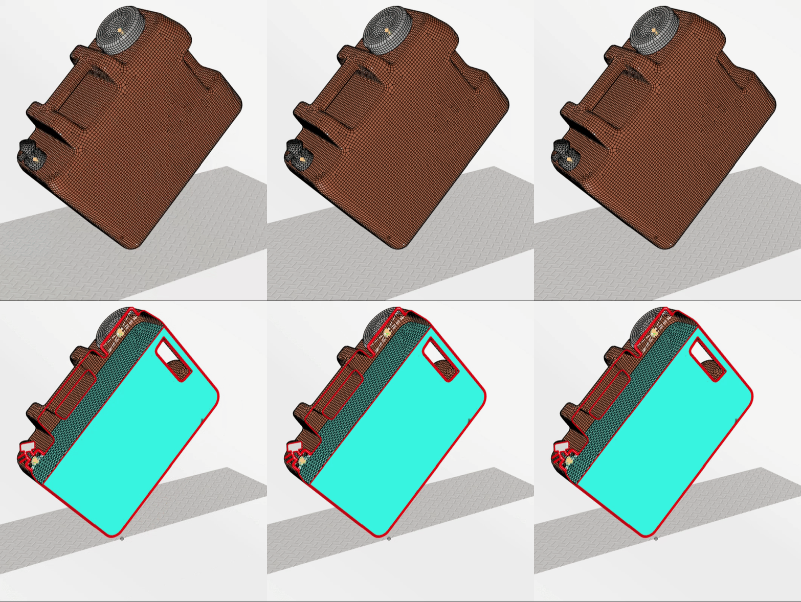
I created an external shell mesh approximation with constant thickness to represent the HDPE plastic jug. The front spout and rear cap are also given HDPE material properties; however, they have been discretized using 2nd order tetraheral elements and 1st order hexahedral elements, respectively. Rather than explicitly model the thread geometry, the front spout and rear cap have been adjoined to the main jug at their junctures using 1D-connector elements that have a prescribed stiffness and pull-through force. With this representation for the thread connections, I can get a rudimentary understanding of the likelihood of a detachment of the front spout or rear cap when subjected to the impact condition.

Internal to the jug, I have a representation for the water by using a Smoothed Particle Hydrodynamic (SPH) section control. This SPH section is then assigned a material card representative of room-temperature water as governed by a linear Mie-Grüneisen () equation of state. By taking this approach, I have a representation for the water that can capture both the inertial and volumetric stiffness contributions the water provides to the jug during the drop test.

These representations for the materials and the discretization of the geometries are then applied to a drop-test scenario from 1.83-meters (or about 6-feet). General contact is utilized to ensure the impact is registered properly. Rather than simulate the entire free-fall plus the impact event, I can use basic linear kinematic equations to calculate the initial velocity and start the simulation right before impact onto the rigid floor.

This simulation has been solved twice, where the only variation is the material model considered for the HDPE. We’ll talk more in detail about the differences in the material models later, but for now, we can observe the contrast between the two simulations when viewed side-by-side. In the following animation, a bilinear tangent plasticity model is used on the jug to the left, whereas a rate-dependent Johnson-Cook governs the jug on the right.

Immediately, I can see a pretty stark difference between these two simulations. For starters, a large buckling and indentation event occurred in the simulation on the left. Additionally, the maximum axial force criterion for the front spout connector element was triggered, causing the failure and release of the spout. In short, the simulation on the left appears to have failed the virtual drop test, while the model on the right appears to pass.

As shown from a different angle, we can see the drastic buckling event and permanent deformation in the bilinear tangent plasticity jug (top) as compared to the rate-dependent Johnson-Cook (bottom). Additionally, the history plots show the relative connector displacement for the front spout and rear cap. The top history plot (representative of the bilinear tangent plasticity jug) shows the connector failure just after t=0.015 seconds as indicated by the sharp peak. The bottom history plot (representative of the Johnson-Cook jug) shows that the relative displacement for the thread connector elements does not exceed 0.125mm and is unlikely to fail.

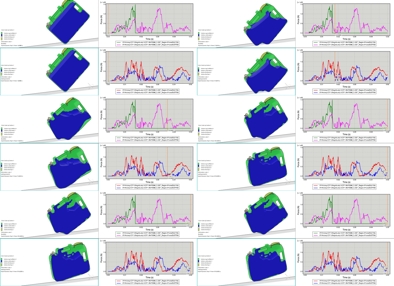
In this final animation, we again place the bilinear tangent plasticity jug and corresponding history results on the top, with the Johnson-Cook versions on the bottom. The field plot animation displays a color-coding of the section material with a cross-section cut down the middle of the jug in order to visualize the sloshing of the water. The history plot animations now show the total axial force within the connectors throughout the duration of the impact event. Again, we can visualize the failure of the top simulation’s front-spout connector element due to the sharp rise and fall around t=0.015 seconds.

There is a large difference in the resulting interpretation of the two simulations we have reviewed. One simulation seems to have passed the virtual drop test, whereas the other failed on several accounts. Again, the only difference between these two models is the representation for the HDPE material card. One simulation utilized a bilinear tangent-plasticity model, whereas the other utilized a slightly more sophisticated strain-rate dependent Johnson-Cook plasticity card. The following image depicts the two material cards shown alongside the test data used to calibrate the rate-dependent Johnson-Cook model.

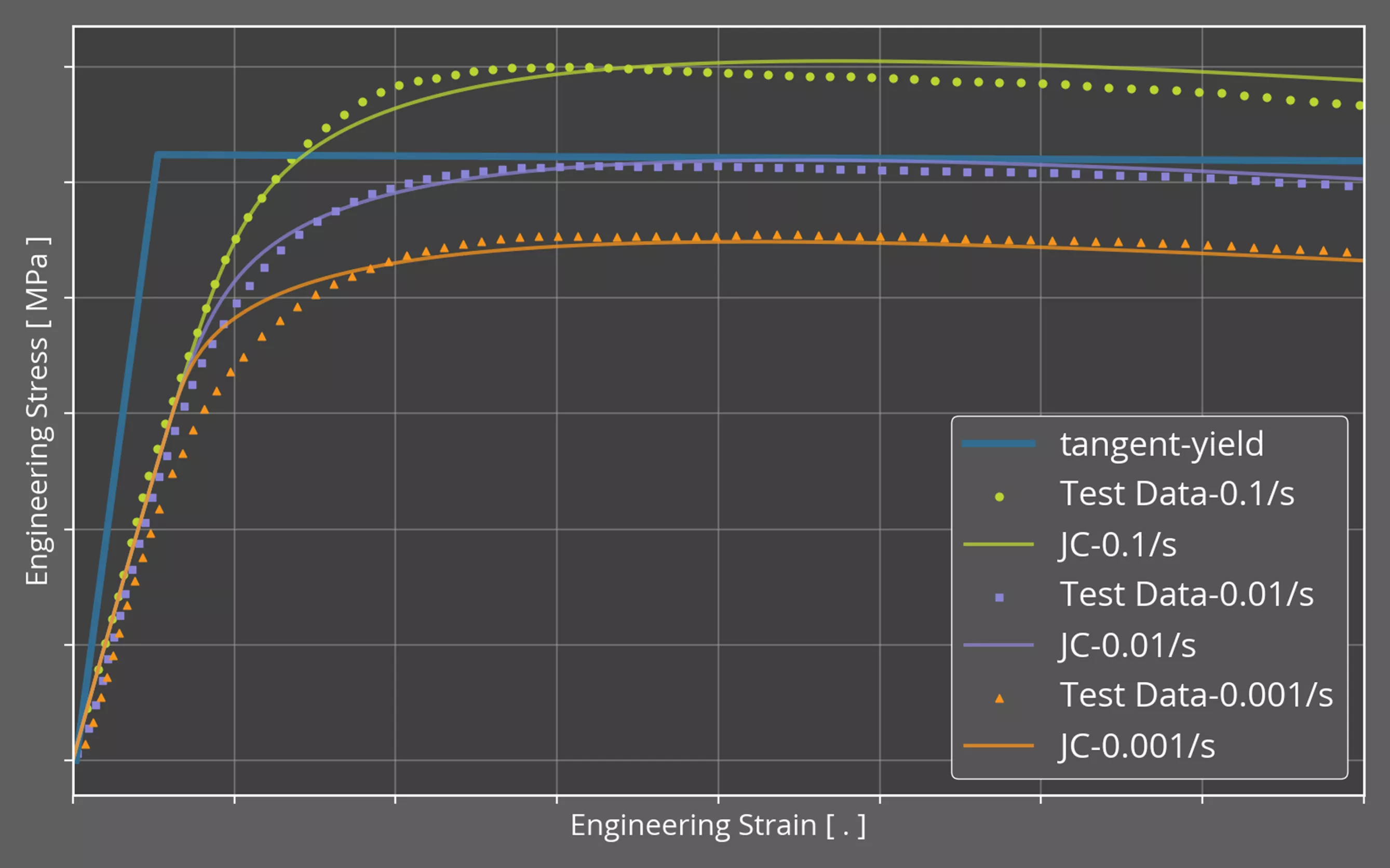
For this demonstration, we’ve approached the material model development in two manners. The first approach involves the collection of averaged material properties from MatWeb, an online material property database. These properties are represented in the “tangent-yield” curve and are sourced from the averaged values across several HDPE, injection molded records. Given that we only have access to the yield stress and ultimate tensile stress, this creates a bilinear material model.

In contrast, the second approach sourced material testing curves from a relevant publication from the Nanjing University of Science and Technology. This approach is beneficial as it allows us to capture some strain-rate dependency of the material; however, it should be noted that for many materials, environmental factors, material processing methods, and other variations can cause discrepancies between your sourced data and your physical product. It is always recommended to seek out material testing at relevant temperatures/strain-rates with samples taken from your supplier in order to minimize the discrepancy between the material properties in reality and your simulation’s representation of the material properties.

With those caveats addressed, we can now look at the Material Calibration app from the 3DEXPERIENCE Platform in order to show how we translate these three strain-rate dependent curves into a single material card. The temperature-independent, strain-rate dependent Johnson-Cook plastic hardening model that we’ll be calibrating in the next section takes the following form:

3DEXPERIENCE Material Calibration App

In order to calibrate our HDPE material to the three stress-strain curves, we’ll start by loading the test data into the application. The 3DEXPERIENCE Material Calibration app supports test data in the form of Excel workbooks (.xslx) or delimited text files (.txt or .csv).

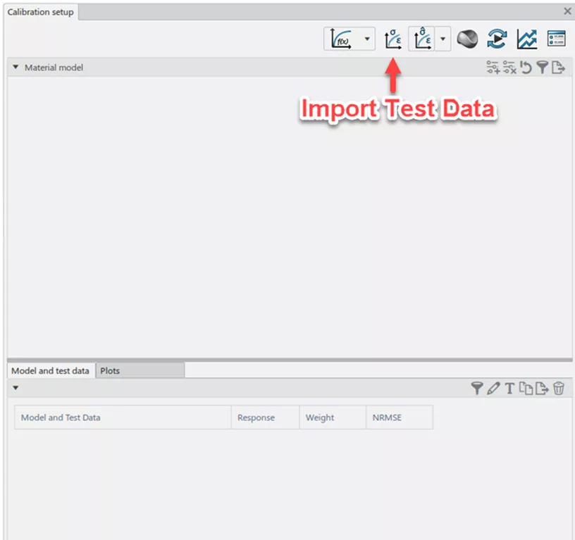
After selecting the .csv file containing the 0.01/s strain-rate data, the following dialogue box appears to guide the import of data. I'll repeat the following steps three times, once for each of the three curves.

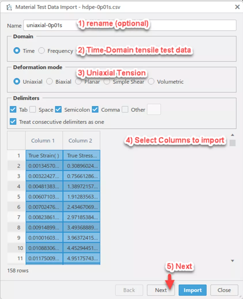
It is recommended to rename the dataset in order to distinguish the curves from one another down the line. Following that, we’ll verify that the options for a time-domain uniaxial test are selected. Options for Biaxial, Planar, and Volumetric will be more important for users looking to calibrate nearly incompressible hyperelastic materials. Next, I’ll click the “Column 1” and “Column 2” headers to indicate that I want to import the data in these fields. With them selected in the data-preview field at the bottom, I’ll hit Next to continue.

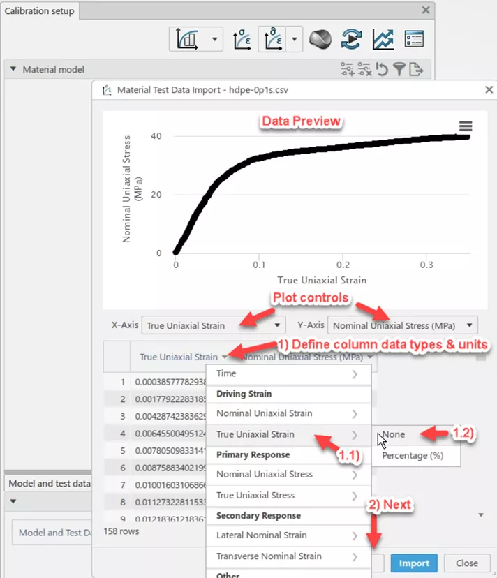
On the second page of the test data import workflow, at the top is a preview of the data. Using the plot controls, you can redefine the variable to be used for the x & y axis if need be.

3DEXPERIENCE will prescribe a datatype to each of the imported columns. In most cases, this will be stress or strain in either the nominal (aka engineering) or true form. In this case, the data we loaded was in the form of true stress and true strain. While selecting the datatype, the user can also indicate what units the stress/strain are in. These values include unitless and percentage for strain, and a wider variety of units for stress including psi, psf, MPa, and more.

If your dataset captured time as an output quantity during the physical experiment, 3DEXPERIENCE can also associate a time value with each of the stress-strain pairs. This time vector can be used directly in the material calibration for time-dependent or strain-rate dependent properties. If time wasn’t directly measured as part of the data set (like in this example), the following page of the test data import workflow can recreate the time vector for you.

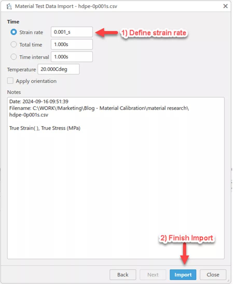
Because our test data did not include a time vector, we can recreate one using a constant strain-rate value. Alternatively, we can define the time vector using either the total time or the interval of time between each data point. This final page of the test data import workflow allows us to denote temperature conditions or material orientations, should we be interested in calibrating thermally-dependent or directionally-dependent material properties down the line.

Now, with all three test data curves imported into the Material Calibration application, the primary dialogue box should look similar to the following:

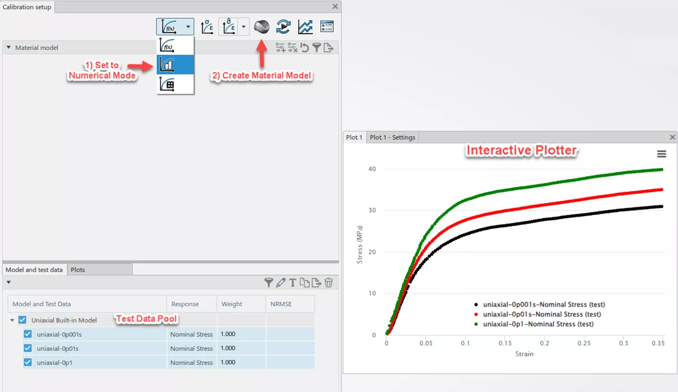
At the bottom of the screen exists the test data pool, organized by deformation mode. Given that I've only included uniaxial tension data, I have only one section. Test data to be considered during the calibration routine is highlighted in blue, and the positive checkbox is selected to the left. On the right-hand side of the image is a view of the interactive plotter showing the three curves in their true stress-strain form.

At this point, let's consider the calibration routines available. The first choice of which will be the selection of a calibration mode that will influence both the material models available for calibration, as well as the overall speed of the calibration.

Analytical Mode is only applicable for hyperelastic and hyperfoam materials; however, it is the fastest of the three because it involves solving for an optimum set of material parameters based on the analytical derivative of the strain energy potential function associated with the chosen material model.

The next, and most commonly used mode, is the Numerical Mode. In this mode, we interface directly with the material subroutines of Abaqus/Standard, passing in the current model parameter values and receiving a response stress-strain curve. This input-response loop is then used in conjunction with a chosen multi-variate optimization algorithm (Hooke-Jeeves, Conjugate Gradient, Particle Swarm, etc.). The Numerical Mode is a computationally efficient optimization method with potentially hundreds of parameter evaluations occurring in seconds. While not quite as fast as Analytical Mode, the support for a wider array of material models makes Numerical Mode the most general-purpose mode of the three.

The final mode is FE-Based Mode, where rather than interfacing solely with the material subroutine in Abaqus/Standard, a full simulation is performed in each parameter evaluation. Each parameter evaluation is based on a user-provided Abaqus input deck (*.inp) or a 3DEXPERIENCE physics simulation object that has been previously created. The FE-Based Mode allows for the recreation of the testing geometry, as well as the calibration of material parameters with respect to kinematic (Force-Displacement) relationships rather than stress-strain alone.  This makes FE-Based the most flexible of the three modes in terms of the physics and material models that can be represented; however, each parameter evaluation will require a full run of the simulation. This then leads to the longest run-times in order to find an optimum set of material parameters.

For our example, I'll stick with the general-purpose Numerical Mode and select the option to create a material model. The following image provides an overview of the many material models available for calibration using Numerical Mode.

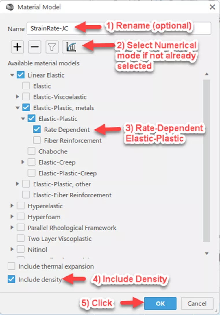
To configure the material model for calibration, I'll first provide a name to be associated with the resulting material. Following that, select Numerical Mode if not already selected. Then for a rate-dependent Johnson-Cook model, I'll expand the model tree options for Linear Elastic  Elastic-Plastic, metals  Elastic Plastic, and select Rate Dependent. Finally, because I'll ultimately be using this material card in an Abaqus/Explicit drop-test, I'll need to include considerations for mass density. This will not influence the calibration of the Johnson-Cook model but will be necessary when it comes time to export it down the line. Lastly, click OK to create the material model.

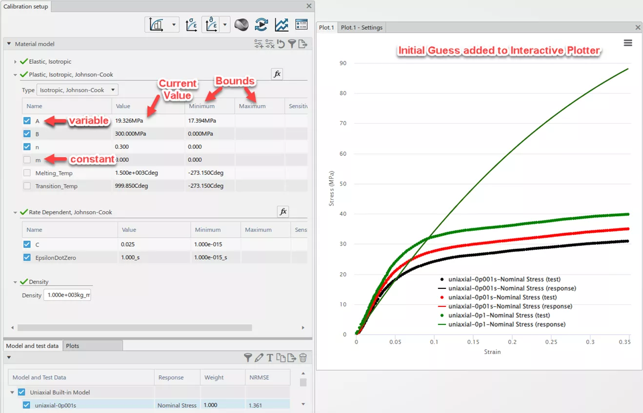
The Calibration Setup page should look similar to the image above. To begin with, the Material Calibration app will provide an initial guess for the material parameters and plot the result on the interactive plotter. In this case, the initial guess for the parameter B appears too high. To indicate that a value is to be modified and ultimately optimized, the user must tick the checkbox on the column next to the parameter name. If the checkbox is blank, the parameter will be kept constant throughout the optimization run.

At this point, it can be helpful to change the values in the Value column in order to observe each parameter’s effect on the resulting curve. This can give the user some insight into what a proper set of bounds should be for each parameter, as well as what would qualify as a reasonable initial value for the optimization. Many gradient-based multi-variate optimizers suffer from a tendency to find localized minima in the parameter space, rather than the global minimum. In these cases, the initial value for the optimization can influence the optimizer’s performance and ability to find a reasonable solution.

In the following image, note the bounds for each parameter that have been specified, as well as which parameters have been activated for the calibration run.

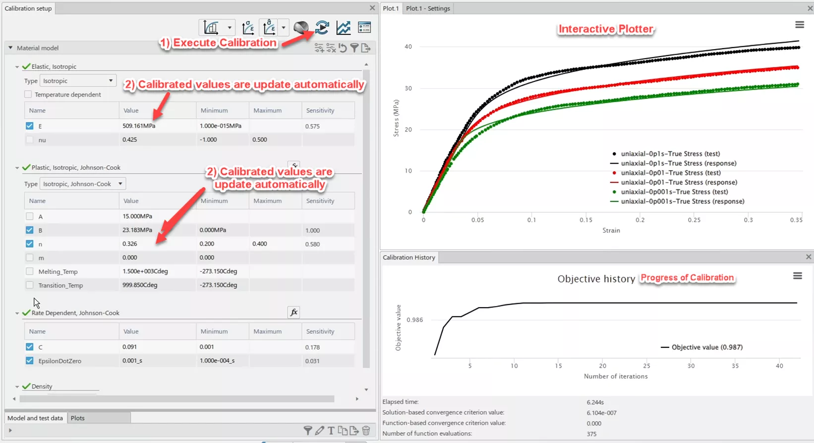
For this calibration, the Material Calibration app modifies values of E, B, n, C, and EpsilonDotZero in order to traverse the parameter space. A Coefficient of Determination (R2) has been utilized to grade the accuracy of each evaluation with respect to the test data. Thus, the chosen optimization algorithm (Nelder-Mead) searches for a parameter set that maximizes the objective value, where a 1.00 value would indicate a perfect fit.

This calibration took approximately 6 seconds and resulted in a parameter set for the Johnson-Cook model that exhibits an R2 value of 0.987 when compared to the three curves from the data pool. From a qualitative perspective, the solid response curves on the previous image’s interactive plotter generally follow the behavior of the scatter plot of test data. There exists some discrepancy in the very low strain-rate data set around the yield point; however, given that we’re ultimately seeking to recreate an impact scenario, the higher strain-rate data will be more influential.

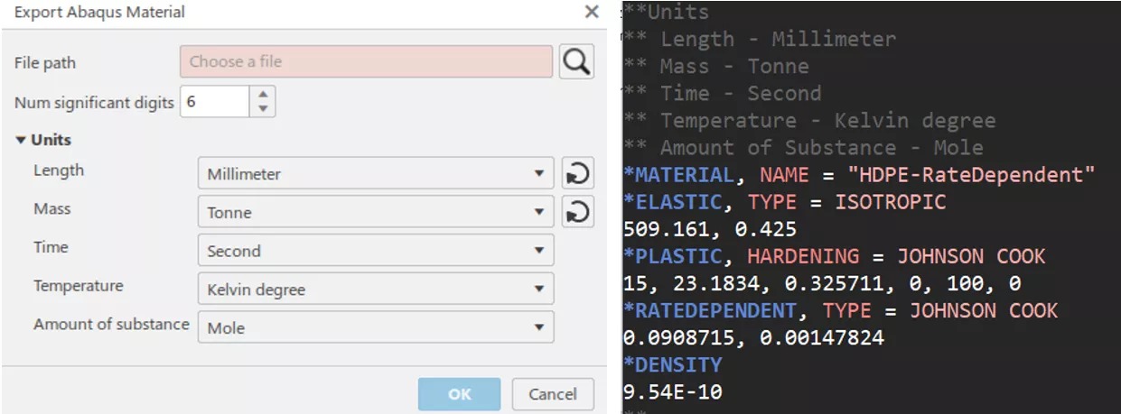
After running the calibration and evaluating the resulting fit, we can now look into exporting the material model. If you plan to build your simulation in the 3DExperience platform using the structural analysis roles (SSU or SYE), you can save the model directly to your tenant’s material database. Alternatively, if you plan on using the established product Abaqus/Explicit, you can export a material card to your machine in whichever unit system you prefer.

Final Thoughts

Through this example, I've demonstrated the importance of adequate material testing and material model development. Simply utilizing generic, averaged material properties from a datasheet can lead to large discrepancies in your simulation’s ability to represent a real-world scenario. If you wish to get the most out of your simulation software, you must investigate material testing that is representative of your product, its manufacturing history, and the environmental factors that influence its material properties.

This workflow has shown how you can easily translate your collected material test data into a form that is usable in your physics simulation. However, there is no “one-size-fits-all” approach to material modeling, and each model will have its strengths, assumptions, and limitations. The Johnson-Cook model utilized in this demonstration was primarily chosen due to its low parameter count and relatively simple governing equation. The real power the 3DEXPERIENCE Material Calibration app gives analysts is the ability to quickly compare the relative performance of multiple similar material models. Reading the documentation to understand the assumptions associated with a material model will always be recommended, but being able to see the response stress-strain curve updated in real time can help build the intuition needed in discerning which model is most applicable for your material.

If this sort of discussion is interesting to you, or you’d like to learn more about the Material Calibration app, one of the best resources can be found in the SIMULIA Community Wiki Page (3DS login required).

Related Articles

Structural FEA for Beginners: 5 Stages of Simulation-Driven Design

Advancing Engineering Simplicity: SIMULIA’s New Unified Licensing Model

Intro to CAD-Connected Composites FEA: A Game-Changer for Composites Design

Enhancing EV Connector Design Using Abaqus FEA

How to Run Abaqus Simulations on the Cloud with the 3DEXPERIENCE Platform

VIEW ALL SIMULATION ARTICLES