Rainflow Counting in SOLIDWORKS Simulation Explained

When performing a Variable Amplitude Time History Fatigue Study in SOLIDWORKS Simulation, a user can view a Rainflow Matrix. What this matrix is and how it’s made may be a question you need to answer. If that is the case, look no further. Rainflow counting is used when performing Variable Amplitude Fatigue studies. In essence, Rainflow counting takes the raw load data and converts it to an equivalent set of constant amplitude stress reversals. It is the industry standard for simplifying the data, so we don’t have to run a full nonlinear dynamic simulation on data like the one shown below.

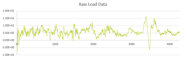
This would be cumbersome to set up, and the computation time is prohibitive for most users.

How Rainflow Counting Works in SOLIDWORKS Simulation 

Rainflow Counting in SOLIDWORKS Simulation performs four functions to streamline the data. 

1. Hysteresis filtering removes any load cycles the user deems too small to matter as a percentage of the maximum range.
2. Peak and Valley filtering extracts the peaks and valleys and eliminates the intermediate data points.
3. Binning to reduce the number of stress levels to be analyzed.
4. Counting the cycles using 4-point Counting.

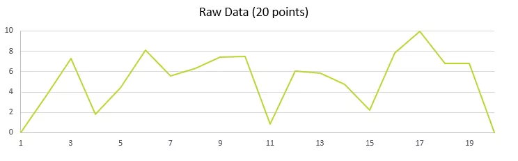
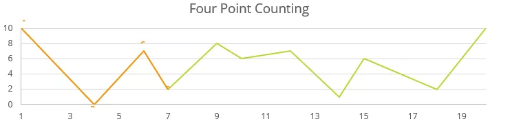
In this example, we will start with the small and simplified raw load data set of 20 points. (Shown below)

Hysteresis Filtering

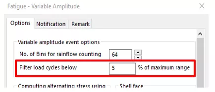
Hysteresis Filtering removes more minor variations and helps to remove noise and inconsequential fluctuations from the data. These minor variations should only be those which will not contribute damage to the degisn. SOLIDWORKS allows the user to choose the filter size by the percentage of the maximum range and removes any data points which fit within that percentage. This setting can be found in the properties of your Variable Amplitude Fatigue study.

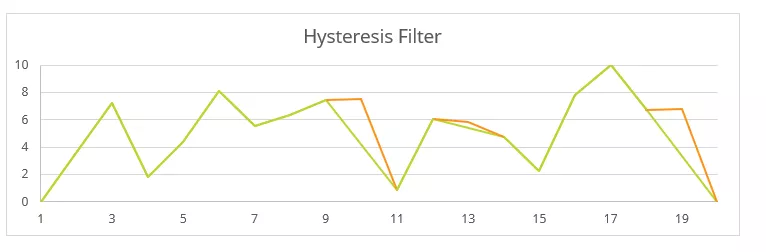
Your value depends on your data and should be chosen carefully. The plot of the data after Hysteresis filtering is shown below in green, with the unfiltered data in orange. 

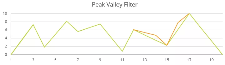
Peak and Valley Filtering

Within a given load/unload cycle, only the maximum and minimum values contribute to the fatigue. Peak and Valley filtering removes all data points that are not these turnaround points. Below I have shown the data with peak and valley filtering. I have shown the data points that were removed in orange. 

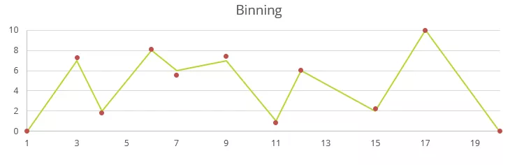
Binning

“Binning” reduces the number of load values (y-axis values) the data can take. Binning moves the y-axis value of the data point to the center of the bin. I have selected 10 bins for simplicity, although the default in SOLIDWORKS Simulation is 25. Having more bins increases the accuracy of the results at the expense of computation time. 

The orange dots show the locations of the previous peaks and valleys; notice how the data below all land directly on the lines and nowhere between.

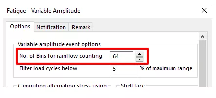
The setting for number of bins, can be found in the same place as the hysteresis filtering option in the study properties.

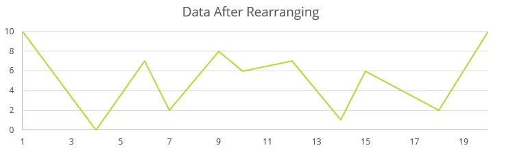
SOLIDWORKS then rearranges the data so that the highest peak is the first and last point in the set. The rearranged set of the first 20 points is shown below.

Four-Point Counting

Four-Point Counting is the heart and soul of the Rainflow Counting method. Now that the superfluous points have been removed, we can begin counting the cycles. This is an iterative process of three steps.

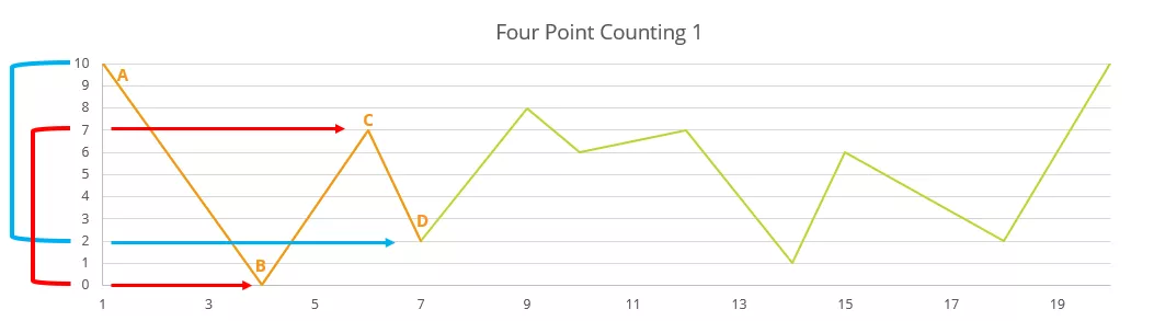
1. Look at four consecutive points and call them A, B, C, and D.
   
   
   
   
2. Test the points to see if the pair of points B-C are bounded by or equal to the pair of points A-D. 
1. If the points pass the test in step 2, count this as a Rainflow cycle and remove points B-C. The cycles are added to Rainflow Matrix explained below. 
2. If the points do not pass the test, move one point forward.
   
   The plots below show two passing and one failing cycle. The orange dots show the inner points B-C, and the green dots show the outer points A-D.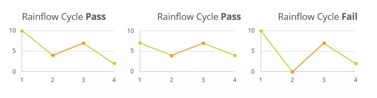
   
   
   
   
3.  Repeat until no Rainflow cycles remain.

Rainflow Matrix

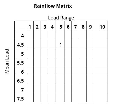
When the midpoints are removed during 4-point Counting, the segment removed is tracked in the Rainflow Matrix. The segment’s range and mean consider only the data’s vertical position (y) and not the time position (x). 

The range of the segment is calculated as |B – C|. 

The mean of the segment is calculated as (B + C) / 2. 

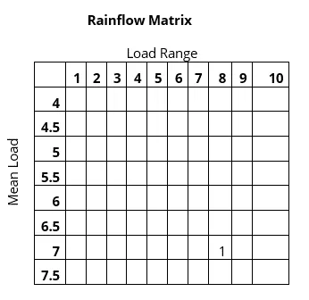
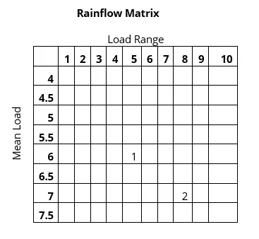
A segment is removed having a Load Range of 8 and a Mean Load of 7; we would insert a “1” in the matrix as shown below. 

Then, if we were to get another segment removed with a Load Range of 5 and a Mean Load of 6, we’d mark the matrix as follows.

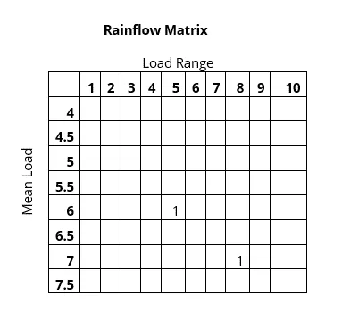
If we removed another segment with a Load Range of 7 and a Mean Load of 8, we would increase the value in that call by 1.

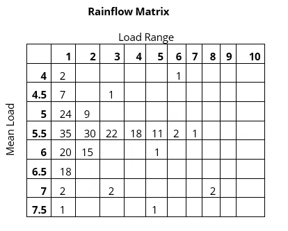
Eventually, we would have a Rainflow matrix that could look something like this.

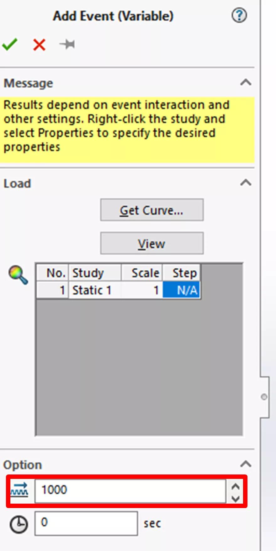
When analyzing a design using Variable Amplitude Time History, we can choose the number of repeats we will put the design through. The Rainflow Matrix represents one pass through a test period or course. We can simulate passing through this same process simply by multiplying the values in each cell by the number of repeats. SOLIDWORKS does this automatically with the “Number of Repeats” option in the definition of the load event below.

Four-Point Counting Example

Let’s work our way through the 20 points we have together. 

Because A-D does not bound B-C, this does not pass the test, and we move on by one point. 

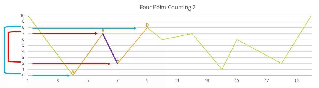
In this case, points A-D bound points B-C, so we count this as a Rainflow Cycle, remove B-C (shown in purple) from the data, and record their values. 

In this example, we went from 7 to 2, giving us a load range of 5 and a mean load of 4.5. So we enter a 1 into that cell. If we were to get another inner segment with a load range of 5 and a mean load of 4.5, we would change the 1 to a 2.

The following GIF shows the process going through the remaining points.

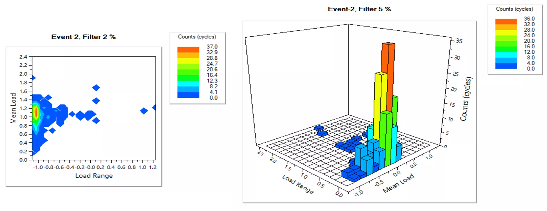
This process would continue throughout the entire data set until only unclosed cycles exist. The end result on actual data will look like the plot below, but instead of numbers, we have colors that indicate the number of cycles (Note: the labels are switched. This is a known issue). SOLIDWORKS also has a 3D version of the same plot.

Conclusion 

Rainflow counting is a powerful method to reduce the computation time when attempting to simulate realistic stress loads on parts or assemblies. The ability to turn chaotic data into sets of cycles allows users to demonstrate how these parts and assemblies will fatigue in the real, non-constant world.

More SOLIDWORKS Simulation Tutorials

Thermal Analysis Using SOLIDWORKS: FEA vs CFD

How to Create Stress-Strain Curves in SOLIDWORKS Simulation

Understanding Thermal Expansion with SOLIDWORKS Simulation

Using Remote Loads in SOLIDWORKS Simulation

Understanding Flaps Using SOLIDWORKS Flow Simulation Parametric Study

VIEW ALL SOLIDWORKS SIMULATION TUTORIALS